39 how to display data labels in excel
How to Use Cell Values for Excel Chart Labels - How-To Geek Select the chart, choose the "Chart Elements" option, click the "Data Labels" arrow, and then "More Options." Uncheck the "Value" box and check the "Value From Cells" box. Select cells C2:C6 to use for the data label range and then click the "OK" button. The values from these cells are now used for the chart data labels. Excel charts: how to move data labels to legend ... @Matt_Fischer-Daly . You can't do that, but you can show a data table below the chart instead of data labels: Click anywhere on the chart. On the Design tab of the ribbon (under Chart Tools), in the Chart Layouts group, click Add Chart Element > Data Table > With Legend Keys (or No Legend Keys if you prefer)
How to display text labels in the X-axis of scatter chart ... Display text labels in X-axis of scatter chart. Actually, there is no way that can display text labels in the X-axis of scatter chart in Excel, but we can create a line chart and make it look like a scatter chart. 1. Select the data you use, and click Insert > Insert Line & Area Chart > Line with Markers to select a line chart. See screenshot: 2.
How to display data labels in excel
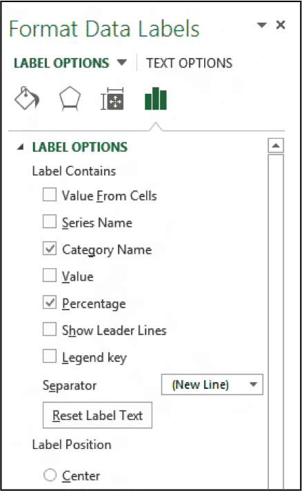
How to show data label in "percentage" instead of ... Select Format Data Labels Select Number in the left column Select Percentage in the popup options In the Format code field set the number of decimal places required and click Add. (Or if the table data in in percentage format then you can select Link to source.) Click OK Regards, OssieMac Report abuse 8 people found this reply helpful · Excel 2010: Show Data Labels In Chart - AddictiveTips To enable data labels in chart, select the chart and head over to Chart Tools Layout tab, from Labels group, under Data Labels options, select a position. It will show Data labels at specified position. Likewise, from Data Labels pull-down menu, you can change the position of data labels and access other advance options. Change the format of data labels in a chart To get there, after adding your data labels, select the data label to format, and then click Chart Elements > Data Labels > More Options. To go to the appropriate area, click one of the four icons ( Fill & Line, Effects, Size & Properties ( Layout & Properties in Outlook or Word), or Label Options) shown here.
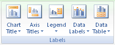
How to display data labels in excel. Outside End Data Label for a Column Chart - ExcelTips (ribbon) Outside End Data Label for a Column Chart. When Rod tries to add data labels to a column chart (Chart Design | Add Chart Element [in the Chart Layouts group] | Data Labels in newer versions of Excel or Chart Tools | Layout | Data Labels in older versions of Excel) the options displayed are None, Center, Inside End, and Inside Base. Format Data Labels in Excel- Instructions - TeachUcomp, Inc. To do this, click the "Format" tab within the "Chart Tools" contextual tab in the Ribbon. Then select the data labels to format from the "Chart Elements" drop-down in the "Current Selection" button group. Then click the "Format Selection" button that appears below the drop-down menu in the same area. Move data labels - support.microsoft.com Right-click the selection > Chart Elements > Data Labels arrow, and select the placement option you want. Different options are available for different chart types. For example, you can place data labels outside of the data points in a pie chart but not in a column chart. Change the format of data labels in a chart To get there, after adding your data labels, select the data label to format, and then click Chart Elements > Data Labels > More Options. To go to the appropriate area, click one of the four icons ( Fill & Line, Effects, Size & Properties ( Layout & Properties in Outlook or Word), or Label Options) shown here.
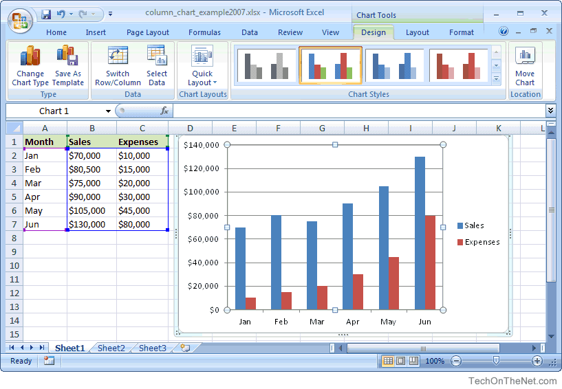
Adding Data Labels to Your Chart (Microsoft Excel) To add data labels in Excel 2013 or Excel 2016, follow these steps: Activate the chart by clicking on it, if necessary. Make sure the Design tab of the ribbon is displayed. (This will appear when the chart is selected.) Click the Add Chart Element drop-down list. Select the Data Labels tool. Custom Chart Data Labels In Excel With Formulas Follow the steps below to create the custom data labels. Select the chart label you want to change. In the formula-bar hit = (equals), select the cell reference containing your chart label's data. In this case, the first label is in cell E2. Finally, repeat for all your chart laebls. Excel tutorial: How to use data labels Generally, the easiest way to show data labels to use the chart elements menu. When you check the box, you'll see data labels appear in the chart. If you have more than one data series, you can select a series first, then turn on data labels for that series only. You can even select a single bar, and show just one data label. How to add data labels from different column in an Excel ... Click any data label to select all data labels, and then click the specified data label to select it only in the chart. 3. Go to the formula bar, type =, select the corresponding cell in the different column, and press the Enter key. See screenshot: 4. Repeat the above 2 - 3 steps to add data labels from the different column for other data points.
Chart: Display alternative values as Data Labels or Data ... Below is my excel chart. I would like to add a "data labels" or "data callouts" As you can see the line is displaying the data from Actual X and Y, but I want to display the DEV values on this line. How can do it? Either any setting or macro code will be much appreicated. Thanks for your time~ Click to expand... for Excel 2013 and up: How to Add Data Labels to an Excel 2010 Chart - dummies On the Chart Tools Layout tab, click Data Labels→More Data Label Options. The Format Data Labels dialog box appears. You can use the options on the Label Options, Number, Fill, Border Color, Border Styles, Shadow, Glow and Soft Edges, 3-D Format, and Alignment tabs to customize the appearance and position of the data labels. Find, label and highlight a certain data point in Excel ... Select the Data Labels box and choose where to position the label. By default, Excel shows one numeric value for the label, y value in our case. To display both x and y values, right-click the label, click Format Data Labels…, select the X Value and Y value boxes, and set the Separator of your choosing: Label the data point by name Quick Tip: Excel 2013 offers flexible data labels ... right-click and choose Insert Data Label Field. In the next dialog, select [Cell] Choose Cell. When Excel displays the source dialog, click the cell that contains the MIN () function, and click OK....
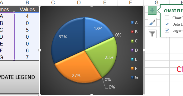
Do My Excel Blog: How to hide the zero percent labels in an Excel pie chart
Edit titles or data labels in a chart - support.microsoft.com The first click selects the data labels for the whole data series, and the second click selects the individual data label. Right-click the data label, and then click Format Data Label or Format Data Labels. Click Label Options if it's not selected, and then select the Reset Label Text check box. Top of Page

32 What Is Data Label In Excel - Labels Design Ideas 2020
How to use data labels in a chart - YouTube Excel charts have a flexible system to display values called "data labels". Data labels are a classic example a "simple" Excel feature with a huge range of o...
How to Create Pivot Tables in Microsoft Excel
How to add or move data labels in Excel chart? 2. Then click the Chart Elements, and check Data Labels, then you can click the arrow to choose an option about the data labels in the sub menu. See screenshot: In Excel 2010 or 2007. 1. click on the chart to show the Layout tab in the Chart Tools group. See screenshot: 2. Then click Data Labels, and select one type of data labels as you need ...
Format Data Labels in Excel 2013- Tutorial - TeachUcomp, Inc.
Datalabels formatter - animadigomma.it The Nordic region is like the rest of Europe in terms of ageing, albeit doing so at a slower pace than the EU average. Support and feedback. Series[1] data label should display count with green color. SeriesCollection(1). When I create a Sunburst chart, I can select the data labels and manually increase/decrease font size via the ribbon.

Format Data Labels in Excel- Instructions - TeachUcomp, Inc.
How to hide zero data labels in chart in Excel? - ExtendOffice In the Format Data Labelsdialog, Click Numberin left pane, then selectCustom from the Categorylist box, and type #""into the Format Codetext box, and click Addbutton to add it to Typelist box. See screenshot: 3. Click Closebutton to close the dialog. Then you can see all zero data labels are hidden.

How to Create a MS Excel 2010 Pivot Table – An Introduction | Technical Communication Center ...
Add or remove data labels in a chart - support.microsoft.com Right-click the data series or data label to display more data for, and then click Format Data Labels. Click Label Options and under Label Contains, select the Values From Cells checkbox. When the Data Label Range dialog box appears, go back to the spreadsheet and select the range for which you want the cell values to display as data labels.
Add or remove data labels in a chart - Office Support
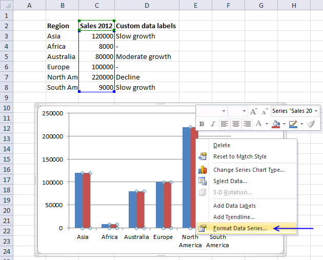
How to Change Excel Chart Data Labels to Custom Values? Now, click on any data label. This will select "all" data labels. Now click once again. At this point excel will select only one data label. Go to Formula bar, press = and point to the cell where the data label for that chart data point is defined. Repeat the process for all other data labels, one after another. See the screencast. Points to note:
create excel spreadsheet for your data for $5 - SEOClerks
Excel Charts: Dynamic Label positioning of line series To see the label for the Budget series, perform the following: Select your chart and go to the Format tab, click on the drop-down menu at the upper left-hand portion and select Series "Budget". Go to Layout tab, select Data Labels > Right. Right mouse click on the data label displayed on the chart. Select Format Data Labels.

How to create Custom Data Labels in Excel Charts – Efficiency 365
How to Customize Your Excel Pivot Chart Data Labels - dummies The Data Labels command on the Design tab's Add Chart Element menu in Excel allows you to label data markers with values from your pivot table. When you click the command button, Excel displays a menu with commands corresponding to locations for the data labels: None, Center, Left, Right, Above, and Below. None signifies that no data labels should be added to the chart and Show signifies ...

Microsoft Excel Tutorials: The Chart Layout Panels
Change the format of data labels in a chart To get there, after adding your data labels, select the data label to format, and then click Chart Elements > Data Labels > More Options. To go to the appropriate area, click one of the four icons ( Fill & Line, Effects, Size & Properties ( Layout & Properties in Outlook or Word), or Label Options) shown here.

How To Show Or Hide Data Labels On MS Excel? | My Windows Hub
Excel 2010: Show Data Labels In Chart - AddictiveTips To enable data labels in chart, select the chart and head over to Chart Tools Layout tab, from Labels group, under Data Labels options, select a position. It will show Data labels at specified position. Likewise, from Data Labels pull-down menu, you can change the position of data labels and access other advance options.

Adobe Using RoboHelp (2017 Release) Robo Help 2017 User Guide Ug En
How to show data label in "percentage" instead of ... Select Format Data Labels Select Number in the left column Select Percentage in the popup options In the Format code field set the number of decimal places required and click Add. (Or if the table data in in percentage format then you can select Link to source.) Click OK Regards, OssieMac Report abuse 8 people found this reply helpful ·
Custom data labels in a chart | Get Digital Help - Microsoft Excel resource

Microsoft Excel Tutorials: The Chart Layout Panels
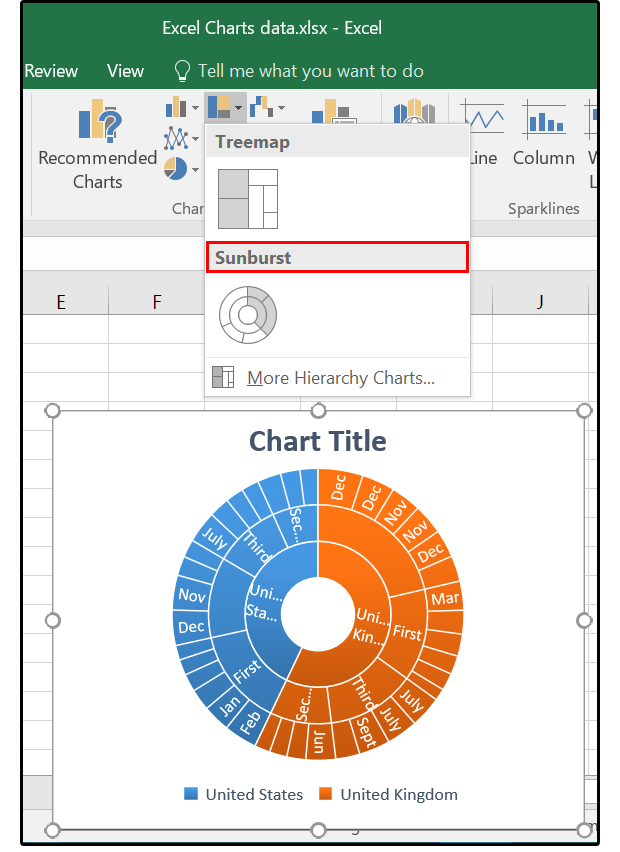
What to do with Excel 2016's new chart styles: Treemap, Sunburst, and Box & Whisker | PCWorld

How to Create a Risk Heatmap in Excel - Part 2 - Risk Management Guru
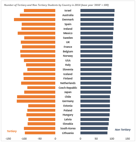
Excel Dot Plots and other charts to display students data

How to Add Data Labels in Excel - Excelchat | Excelchat
Post a Comment for "39 how to display data labels in excel"